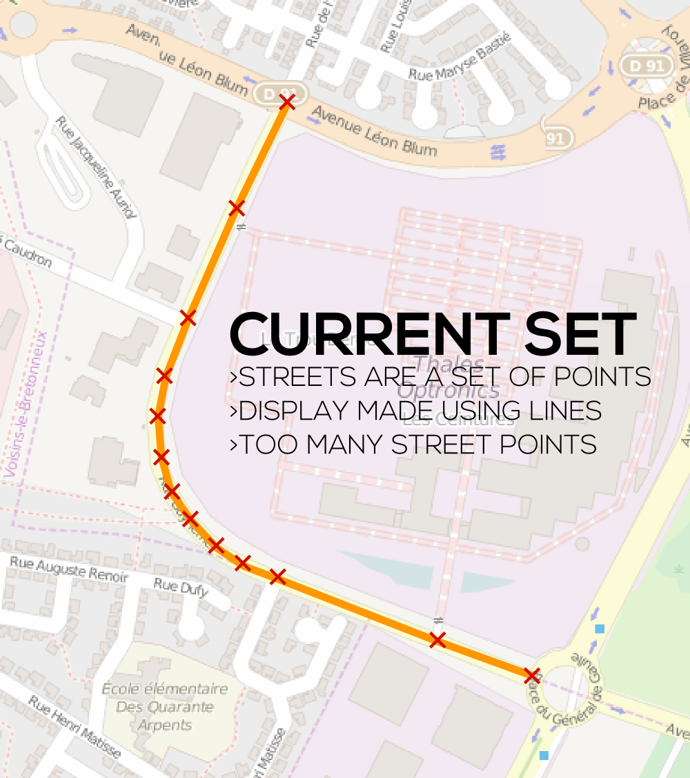
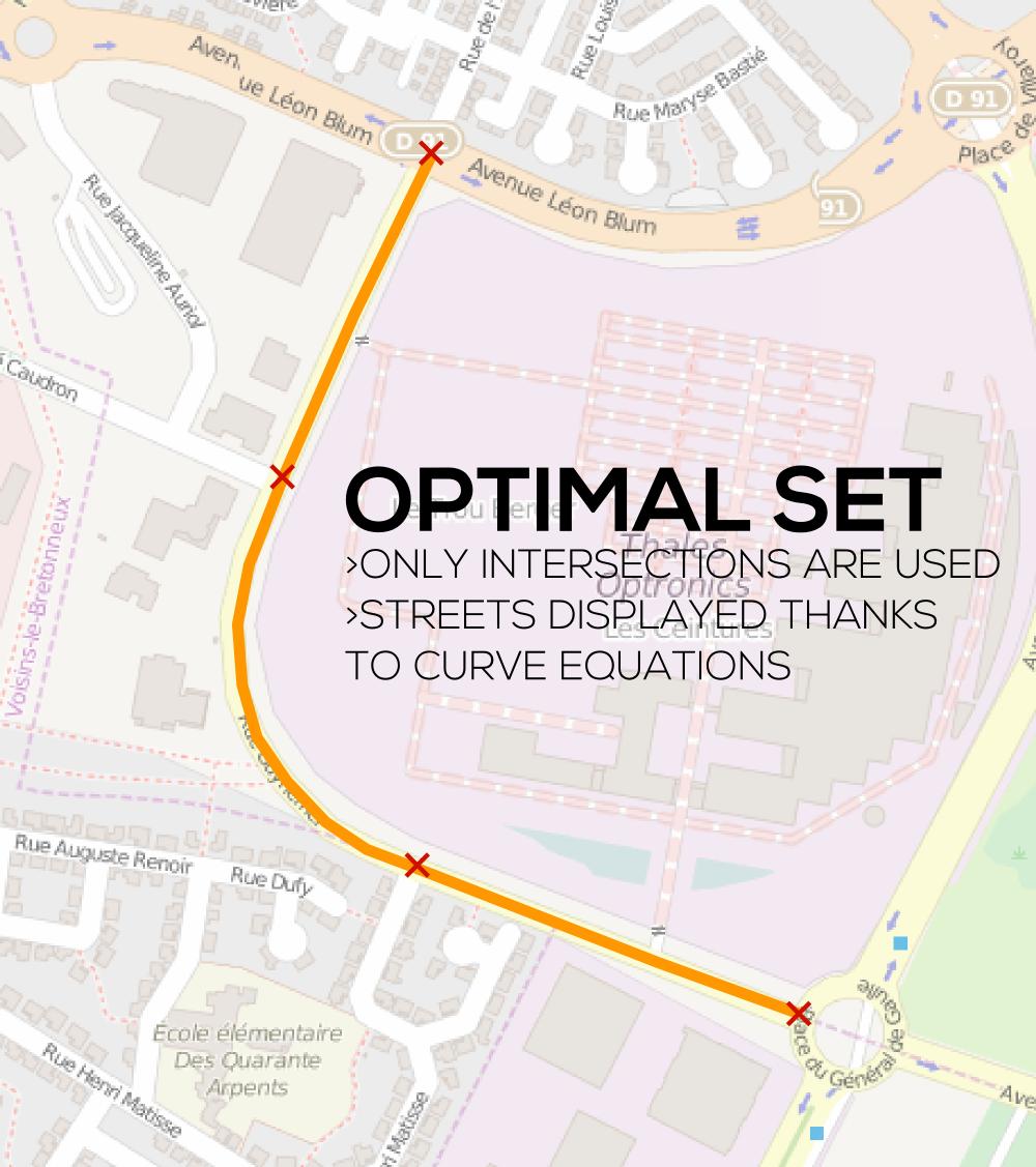
Streets can be pretty funky, with plenty of twists and turns. This can make it hard - or impossible - to describe one by a function of the form \$y = f(x)\$, where \$x\$ and \$y\$ are Cartesian coordinates. Polar coordinates, too, will often fail, no matter where you choose the origin. Therefore, I think your best bet is to create a parametric curve - that is, a relationship so that any point \$(x,y)\$ can be represented by functions of some parameter \$t\$:
$$(x,y) = (f(t), g(t))$$
When you're doing some sort of curve fitting like this, it's best to make \$t\$ proportional to the arc length \$s\$, which tells you where on the curve you are. You can then treat \$t\$ as the time it takes to move along the curve with some constant velocity (usually set to 1).
Step 1: A good approximation
Let's say you have a series of ten points \$\{p_1,p_2,p_3,p_4,p_5,p_6,p_7,p_8,p_9,p_{10}\}\$ on your grid, each one with coordinates \$p_j=(x_j,y_j)\$. You want to create a curve \$P(t)\$ that contains them all. The curve starts at \$p_1\$, and goes from \$p_j\$ to \$p_{(j+1)}\$ until it reaches \$p_{10}\$, where it stops.
We need to figure out the time at which a person traveling on the curve reaches the next point, i.e. how far apart two points are. If they're close enough together, then a linear approximation is enough. In pseudocode:
$$p_1 = (x_1,y_1)$$
$$p_2 = (x_2,y_2)$$
$$d_x = x_2 - x_1$$
$$d_y = y_2 - y_1$$
$$dist = \sqrt{d_x^2+d_y^2}$$
We do this for each two points. If \$P(t_1) = p_1\$, then \$P(t_2 - t_1) = p_2\$, where \$t_2\$ is the linear distance between \$p_1\$ and \$p_2\$. We can set \$t_1 = 0\$, if we want, for the sake of simplicity - assuming \$p_1\$ is one of the endpoints.
After we've done this for all the points, we have three sets of numbers:
$$\begin{align}T =& \{t_1,t_2,t_3,t_4,t_5,t_6,t_7,t_8,t_9,t_{10}\}\\
X =& \{x_1,x_2,x_3,x_4,x_5,x_6,x_7,x_8,x_9,x_{10}\} \\
Y =& \{y_1,y_2,y_3,y_4,y_5,y_6,y_7,y_8,y_9,y_{10}\}\end{align}$$
and so at \$t=t_j\$, the curve is at point \$p_j(x_j,y_j)\$. Now we can interpolate. You can construct two Lagrange polynomials1, one each for the \$x\$ and \$y\$ coordinates, each in terms of \$t\$. The formula is simple enough, although it's obviously harder to do by hand.
We now have a parametric curve that describes all the points.
But wait! That still requires a lot of coefficients, and we're trying to reduce that. So why did we even do this?
Step 2: Remove some points.
Let's say we only want to use four points. That's reasonable. I'll pick the endpoints and two others: \$\{p_1,p_4,p_7,p_{10}\}\$. Now, we can do the same thing as before. In fact, we could do the same interpolation we did in Step 1, by just finding the linear distance. And that's fine if you have a curve that only deviates a little from a straight line during each segment. However, that's often not the case. By simply finding the shortest distance between \$p_4\$ and \$p_7\$, we'd think that the two are a lot closer together, making the curve a lot different.
Therefore, we take what we did from step one. We find the length between these two points based on our interpolated curve \$P\$ that uses all ten. This can be done by just finding the arc length. I'd recommend using numerical methods for this. We then have three sets:
$$\begin{align}T =& \{t_1',t_4',t_7',t_{10}'\}\\
X =& \{x_1,x_4,x_7,x_{10}\} \\
Y =& \{y_1,y_4,y_7,y_{10}\}\end{align}$$
I use the primes to show that the times we've found are different from what we did in step one. They may be more accurate. Now we do the same sort of interpolation, just with four points.
We now have a parametric equation for the curve, using only four points. It's much less accurate than the first equation, but it uses much less data, and it guarantees that the curve will still pass through these four points (that's an issue with polynomial regression - only rarely will a best-fit curve go through any of the points).
Now, we could have skipped Step 1. I know, maybe you're disappointed. As I said before, we could just have used the linear distances between the four points. But that misses most of the finer details of the curve, and if you're shortening a curve from, say, 20 points to 6 points, skipping the first interpolation could really be costly.
1 A Lagrange polynomial (not parameterized) is of the form
$$L(x)=\sum_{i=1}^ny_ik_i(x)$$
where
$$k_i(x)=\prod_{m=0,m\neq i}^n\frac{x-x_m}{x_i-x_m}$$
Here's the reasoning behind Lagrange polynomials (in this case, there is no parameterization - \$y\$ is directly a function of \$x\$). You have \$n\$ points with coordinates \$\{(x_1,y_1),(x_2,y_2), ... ,(x_n,y_n)\}\$. You want to come up with a non-parameterized function \$y = f(x)\$. The simplest way to do that is to come up with a function with \$n\$ terms. At each point \$p_j\$, i.e. when \$x = x_j\$, all but one term - let's call it the jth term - will come to zero, and the remaining term will be equal to \$y_j\$. From there, it's simple to construct the second expression for any point \$p_l\$, and you simply add up \$n\$ terms, each corresponding to a different \$p_l\$, \$x_l\$ and \$y_l\$. This gives you the Lagrange polynomial for your set of points.
In your application of Lagrange polynomials to streets, we've done the same thing - just parametrically.


