Is there a known most efficient version of A* search algorithm?

Question

Is there a known 'most efficient' version of the A* search algorithm? I know some people write papers on the most efficient way to compute common operations, has this been done for A*?

Answer 1

If you don't mind bibliography, take this list as a starting point. It's a series of articles from the Game Programming Gems and the AI Game Programming Wisdom series, with the most relevant ones being:

• Beyond A* - Game Programming Gems 5
• Advanced Pathfinding with Minimal Replanning Cost: Dynamic A Star (D*) - Game Programming Gems 5
• How to Achieve Lightning Fast A* - AI Game Programming Wisdom
• Practical Optimizations for A* Path Generation - AI Game Programming Wisdom
• A* Aesthetic Optimizations - Game Programming Gems
• A* Speed Optimizations - Game Programming Gems

If I remember correctly from what I've read, there's no ultimate version of A* being presented, but rather a series of optimization and improvements you can make to increase its performance or memory usage in specific scenarios.

---

I wanted to add a bit more detail since I own these books, but I won't have access to them until the end of the month. Here's what I can somewhat recall from memory though. First, there are several optimization you can apply while using a regular A* implementation.

The most significant change you can make is simplifying the search space. There are many different ways to represent your search space, each with pros and cons, and choosing the correct one for the job is pretty much the most deciding factor in A* performance. The most common space representations are using a grid, a navigation mesh or a visibility graph.

Tweaking the heuristic can also affect the speed of your pathfinding. For instance, they say that the heuristic has to be admissible (i.e. it never overestimates the actual cost) for A* to find you the best path. But sometimes if you overestimate the heuristic a little it will speed up the search and the paths returned will be similar enough (maybe not perfect every time, but significantly close).

Finally, there are many variations on the algorithm itself to make it work under different circunstances, for instance, just to name a few:

• D* (Dynamic) - Dynamic in the sense that it works under the assumption that the terrain can change even while you're still looking for the path.
• HPA* (Hierarchical) - Uses several layers at different abstraction levels to speed up the search. For instance, an higher level layer may simply connect rooms, while a lower level layer takes care of avoiding obstacles.
• IDA* (Iterative Deepening) - Reduces memory usage in comparison with regular A* by using iterative deepening.

Answer 2

Bit of an old one (stumbled into this searching for something else entirely) but I didn't see Jump Point Search explicitly mentioned.

There's a good article here (which I think is from someone who worked closely on the development of the approach) that describes very well how it works, how to implement it, and why it's faster.

Briefly it works on the notion that you can cull the search space on A* without needing to consult the heuristic, due to the flat (as in space-curvature) nature of grids (examples are 2D, but it works for 3D as well, if properly extended). There's no need to add the node you just came from to the search space, obviously, but there's also no need to add any common neighbors either: it will always be faster to go from the parent to the common neighbor directly than to pass through the current node, so you end up with the following:

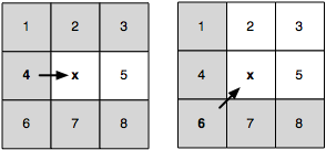
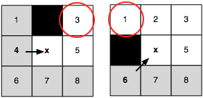
Where the arrow represents parent-to-current, the gray nodes can be ignored, and the white nodes are the new ones that need to be added to the search space. [4,2,3] and [4,x,3] have identical path lengths, but it is excluded as it will already be checked later when expanding from node #2 diagonally (see Figure 3) or earlier (e.g. the parent of node #4).

There are some special-case rules dealing with obstacles (e.g. if in the right half of the above image, if node #4 was impassable, you'd need to include node #1 in addition to 2, 3, and 5):

As well as simply heading in a straight line until an obstacle is reached before adding any nodes to the search space at all (hence the name of the optimization: "jump point" as the code locates virtual "lily pads" that it jumps to as the only important nodes in the path).

Intuitively, the objective is to eliminate symmetries by recursively “jumping over” all nodes which can be reached optimally by a path that does not visit the current node. We stop the recursion when we hit an obstacle or when we find a so-called jump point successor. Jump points are interesting because they have neighbours that cannot be reached by an alternative symmetric path: the optimal path must go through the current node.

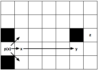
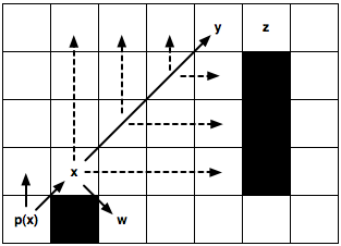
Figure 3: Jumping Examples. Node x is currently being expanded. p(x) is its parent.

(a) We recursively apply the straight pruning rule and identify y as a jump point successor of x. This node is interesting because it has a neighbour z that cannot be reached optimally except by a path that visits x then y. The intermediate nodes are never explicitly generated or even evaluated.

(b) We recursively apply the diagonal pruning rule and identify y as a jump point successor of x. Notice that before each diagonal step we first recurse straight (dashed lines). Only if both straight recursions fail to identify a jump point do we step diagonally again. Node w, which is simply a forced neighbour of x, is generated as normal.

Even without the recursion, the simple pruning and forced-neighbors rules improve the performance of A* dramatically and are incredibly easy to implement. I did it once myself and only had a few minor problems related to pruning the list post-A* so that I could have straight lines through open spaces (rather than diagonal doglegs) that resulted in a very hard to replicate issue where a path tried to prune 90% of its length by going through a wall. It only happened in a very specific setup, only in the one direction, and never managed to figure out why it thought it was ok (project has since been scraped and rebuilt from the ground up).

Answer 3

D* Lite if you want AI that behaves in the way that a human might when exploring a completely new and unknown area, needing no prior knowledge of the map except for the coordinates of start and goal, and which can adapt to a changing map. This algorithm is both conceptually simpler and more efficient than the original D*, effectively obsoleting D*. It's been used in some of the Mars rovers. This algorithm eliminates the typical "omniscient", know-it-all behaviour of AIs we've all seen in games, the ones that move based on a single pre-emptive A* run on a known map.

D* Lite works on an ad hoc basis. It begins by calculating a fairly direct path between the designated goal and start points, working backward from goal to start, not yet knowing the occupancy status of those nodes along the path. It then begins to walk this path, like a pioneer.

This continues until it hits an obstacle on a node which it previously expected to walk through on its way to the goal. As a result of this mishap, it recalculates the remaining path (again backwards from goal to present position) based on the now known obstacle(s) and tries to continue stepping. Each time it find a new obstacle along its path, it recalculates as best it can based on the sum total of its current knowledge. If it follows a path to a dead-end, it will backtrack and seek new routes to goal.

P.S. "Most efficient" depends on your use case. For procedural, changing terrains and where realistic exploration is paramount, D* Lite is "most efficient".

P.P.S. Just like A*, you can also accelerate D* Lite with Jump Point Search, also mentioned here.

---

Generalized Adaptive A* (GAA*) is good where you want a constantly moving target. I've not tried it myself but the linked paper suggests that it is faster than A* and D* Lite etc. for this purpose.

Answer 4

A* is the basic, most widely used, most general purpose graph traversal algorithm. Given a set of nodes, edges, and weights for those edges, a starting node, and an ending node, A* will find the shortest path between the 2 points.

As you must know, many variants on A* exist.

Some of these variants do things like allow for edge weights to change (dynamically "updateable" solution) (D*: The name D* comes from the term "Dynamic A*", because the algorithm behaves like A* except that the arc costs can change as the algorithm runs.).

Algorithms such as LRTA* (learning real time A*) will modify the graph as it explores it, increasing costs of edges that lead to dead ends and the like (hence "learning").