How does A* pathfinding work?

Question

I would like to understand on a fundamental level the way in which A* pathfinding works. Any code or psuedo-code implementations as well as visualizations would be helpful.

Answer 1

Disclaimer

There are tons of code-examples and explanations of A* to be found online. This question has also received lots of great answers with a lot of useful links. In my answer I'll try to provide an illustrated example of the algorithm, which might be easier to understand than code or descriptions.

---

Dijkstra's algorithm

To understand A*, I suggest you first have a look at Dijkstra's algorithm. Let me guide you through the steps Dijkstra's algorithm will perform for a search.

Our start-node is A and we want to find the shortest path to F. Each edge of the graph has a movement cost associated with it (denoted as black digits next to the edges). Our goal is to evaluate the minimal travel cost for each vertex (or node) of the graph until we hit our goal node.

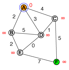
This is our starting point. We have a list nodes to examine, this list currently is:

{ A(0) }

A has a cost of 0, all other nodes are set to infinity (in a typical implementation, this would be something like int.MAX_VALUE or similar).

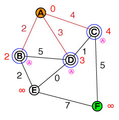
We take the node with the lowest cost from our list of nodes (since our list only contains A, this is our candidate) and visit all its neighbors. We set the cost of each neighbor to:

Cost_of_Edge + Cost_of_previous_Node

and keep track of the previous node (shown as small pink letter below the node). A can be marked as solved (red) now, so that we don't visit it again. Our list of candidates now looks like this:

{ B(2), D(3), C(4) }

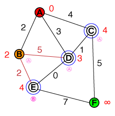
Again, we take the node with the lowest cost from our list (B) and evaluate its neighbors. The path to D is more expensive than the current cost of D, therefore this path can be discarded. E will be added to our list of candidates, which now looks like this:

{ D(3), C(4), E(4) }

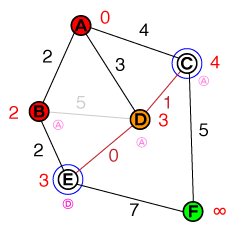
The next node to examine is now D. The connection to C can be discarded, as the path isn't shorter than the existing cost. We did find a shorter path to E though, therefore the cost for E and its previous node will be updated. Our list now looks like this:

{ E(3), C(4) }

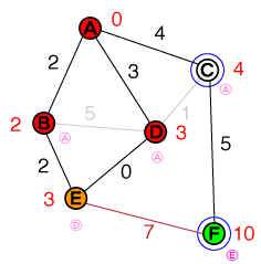
So as we did before, we examine the node with the lowest cost from our list, which is now E. E only has one unsolved neighbor, which is also the target node. The cost to reach the target node is set to 10 and its previous node to E. Our list of candidates now looks like this:

{ C(4), F(10) }

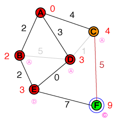
Next we examine C. We can update the cost and previous node for F. Since our list now has F as node with the lowest cost, we're done. Our path can be constructed by backtracking the previous shortest nodes.

---

A* algorithm

So you might wonder why I explained Dijkstra to you instead of the A* algorithm? Well, the only difference is in how you weigh (or sort) your candidates. With Dijkstra it's:

Cost_of_Edge + Cost_of_previous_Node

With A* it's:

Cost_of_Edge + Cost_of_previous_Node + Estimated_Cost_to_reach_Target_from(Node)

Where Estimated_Cost_to_reach_Target_from is commonly called a Heuristic function. This is a function that will try to estimate the cost to reach the target-node. A good heuristic function will achieve that less nodes will have to be visited to find the target. While Dijkstra's algorithm would expand to all sides, A* will (thanks to the heuristic) search in the direction of the target.

Amit's page about heuristics has a good overview over common heuristics.

Answer 2

A* path finding is a best-first type search that uses an additional heuristic.

The first thing you need to do is divide up your search area. For this explanation the map is a square grid of tiles, because most 2D games use a grid of tiles and because that's simple to visualize. Note however that the search area can be broken up in any way you want: a hex grid perhaps, or even arbitrary shapes like Risk. The various map positions are referred to as "nodes" and this algorithm will work any time you have a bunch of nodes to traverse and have defined connections between the nodes.

Anyway, starting at a given starting tile:

• The 8 tiles around the starting tile are "scored" based on a) the cost of moving from the current tile to the next tile (generally 1 for horizontal or vertical movements, sqrt(2) for diagonal movement).

• Each tile is then assigned an additional "heuristic" score--an approximation of the relative worth of moving to each tile. Different heuristics are used, the simplest being the straight-line distance between the centers of the given tile and end tile.

• The current tile is then "closed", and the agent moves to the neighboring tile that is open, has the lowest movement score, and the lowest heuristic score.

• This process is repeated until the goal node is reached, or there are no more open nodes (meaning the agent is blocked).

For diagrams illustrating these steps, refer to this good beginner's tutorial.

There are some improvements that can be made, mainly in improving the heuristic:

• Taking into account terrain differences, roughness, steepness, etc.

• It is also sometimes useful to do a "sweep" across the grid to block out areas of the map that are not efficient paths: a U shape facing the agent, for example. Without a sweep test, the agent would first enter the U, turn around, then leave and go around the edge of the U. A "real" intelligent agent would note the U shaped trap and simply avoid it. Sweeping can help simulate this.

Answer 3

It's far from the best, but this an implementation I did of A* in C++ a few years ago.

It's probably better that I point you to resources than attempt to explain the entire algorithm. Also, as you read through the wiki article, play with the demo and see if you can visualize how it is working. Leave a comment if you have a specific question.

1. A* on Wikipedia
2. A* Java demonstration

Answer 4

You might find ActiveTut's article on Path Finding useful. It goes over both A* and Dijkstra's Algorithm and the differences between them. It's geared toward Flash developers, but it should provide some good insight on the theory even if you don't use Flash.

Answer 5

One thing that's important to visualize when dealing with A* and Dijkstra's Algorithm is that A* is directed; it tries to find the shortest path to a particular point by "guessing" which direction to look. Dijkstra's Algorithm finds the shortest path to /every/ point.

Answer 6

So just as a first statement, A* is at heart a graph exploration algorithm. Usually in games we use either tiles or other world geometry as the graph, but you can use A* for other things. The two ur-algorithms for graph traversal are depth-first-search and breadth-first-search. In DFS you always fully explore down your current branch before looking at siblings of the current node, and in BFS you always look at siblings first and then children. A* tries to find a middle-ground between these where you explore down a branch (so more like DFS) when you are getting closer to the desired goal but sometimes stop and try a sibling if it might have better results down its branch. The actual math is that you keep a list of possible nodes to explore next where each has a "goodness" score indicating how close (in some kind of abstract sense) it is to the goal, lower scores being better (0 would mean you found the goal). You select which to use next by finding the minimum of the score plus the number of nodes away from the root (which is generally the current configuration, or current position in pathfinding). Each time you explore a node you add all its children to this list and then pick the new best one.

Answer 7

On an abstract level, A* works like this:

• You treat the world as a discrete number of connected nodes, eg. a grid, or a graph.
• To find a path across that world, you need to find a list of adjacent 'nodes' within that space, leading from the start to the goal.
• The naïve approach would be this: calculate every possible permutation of nodes that begin with the start node and finish at the end node, and choose the cheapest. This would obviously take forever on all but the tiniest spaces.
• Therefore alternative approaches attempt to use some knowledge about the world to guess which permutations are worth considering first, and to know whether a given solution can be beaten. This estimate is called a heuristic.
• A* requires a heuristic that is admissible. This means that it never overestimates.
  • A good heuristic for pathfinding problems is the Euclidean distance because we know that the shortest route between 2 points is a straight line. This never overestimates the distance in real-world simulations.
• A* begins with the start node, and tries successive permutations of that node plus each neighbour, and its neighbour's neighbours, etc., using the heuristic to decide which permutation to try next.
• At each step, A* looks at the most promising path so far and picks the next neighbouring node that appears to be 'best', based on the distance travelled so far, and the heuristic's estimate of how far would be left to go from that node.
• Because the heuristic never overestimates, and the distance travelled so far is known to be accurate, it will always pick the most optimistic next step.
  • If that next step reaches the goal, you know it has found the shortest route from the last position, because this was the most optimistic guess of the valid ones remaining.
  • If it didn't reach the goal, it is left as a possible point to explore from later. The algorithm now chooses the next most promising possibility, so the logic above still applies.