13
\$\begingroup\$

I've been reading this: http://theory.stanford.edu/~amitp/GameProgramming/Heuristics.html

But there are some things I don't understand, for example the article says to use something like this for pathfinding with diagonal movement:

function heuristic(node) =
    dx = abs(node.x - goal.x)
    dy = abs(node.y - goal.y)
    return D * max(dx, dy)

I don't know how do set D to get a natural looking path like in the article, I set D to the lowest cost between adjacent squares like it said, and I don't know what they meant by the stuff about the heuristic should be 4*D, that does not seem to change any thing.

This is my heuristic function and move function:

def heuristic(self, node, goal):
    D = 5
    dx = abs(node.x - goal.x)
    dy = abs(node.y - goal.y)
    return D * max(dx, dy)

def move_cost(self, current, node):
   cross = abs(current.x - node.x) == 1 and abs(current.y - node.y) == 1
   return 7 if cross else 5

Result:
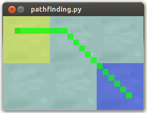
enter image description here

The smooth sailing path we want to happen:
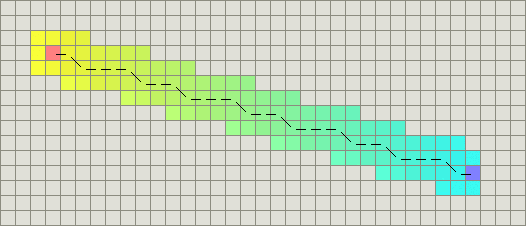
enter image description here

The rest of my code: http://pastebin.com/TL2cEkeX


Update

This is the best solution I have found so far:

def heuristic(node, start, goal):
    dx1 = node.x - goal.x
    dy1 = node.y - goal.y
    dx2 = start.x - goal.x
    dy2 = start.y - goal.y
    cross = abs(dx1*dy2 - dx2*dy1)

    dx3 = abs(dx1)
    dy3 = abs(dy1)

    return 5 + (cross*0.01) * (dx3+dy3) + (sqrt(2)-2) * min(dx3, dy3)

def move_cost(current, node):
    cross = abs(current.x - node.x) == 1 and abs(current.y - node.y) == 1
    return 7 if cross else 5

It produces the desired path from the second pic, but does not handle obstacles very well (tends to crawl on walls) and fails to produce optimal paths sometimes on longer distances.

What are some tweaks and optimizations I can apply to improve it?

\$\endgroup\$
3
  • 2
    \$\begingroup\$ What if you use cartesian distance as your heuristic? \$\endgroup\$
    – Jimmy
    Commented Nov 1, 2013 at 21:25
  • 2
    \$\begingroup\$ here is just an idea, increase the cost of moving from one tile to another for every step agent moves in same direction. \$\endgroup\$
    – Ali1S232
    Commented Nov 1, 2013 at 21:41
  • \$\begingroup\$ @Jimmy I tried sqrt(pow(goal.x - node.x, 2) + pow(goal.y - node.y, 2)) and for my small example path it actually returns the exact same as the picture in my question. \$\endgroup\$ Commented Nov 1, 2013 at 21:47

3 Answers 3

10
\$\begingroup\$

A* gives you the shortest path in the graph. When using a grid as your graph there are often multiple shortest paths. In your first diagram, that is one of the shortest paths. It puts all the axial movements first and all the diagonal movements afterwards. But that's the same length path as if you put all the diagonals first, or if you mixed axial and diagonal movements. These are all equivalently short, and which one A* picks depends on how the code is written and how the graph is represented.

I think what you're wanting is either:

  1. You need to move on the grid, but you want to mix the axial and diagonal steps so that it looks better. One approach is to choose one of the other equally short paths; keep reading that Heuristics page to find “tie breaking”. Another approach is when you're evaluating neighbors, choose randomly which one to evaluate first so that it doesn't always pick one before the other. I do not recommend using Euclidean/Cartesian distance if you want to move on the grid; it's a mismatch that makes A* run slower.
  2. You don't need to move on the grid, and want to move in a straight line. One approach is to straighten out the paths using “string pulling”. You're looking for places where the path turns, and drawing straight lines between those points. Another approach is to apply this to the underlying graph itself. Instead of pathfinding on the grid, pathfind on the key points on the map, and then move along straight lines between those key points. You can see an example here. Yet another approach is the Theta* algorithm.
\$\endgroup\$
2
  • \$\begingroup\$ Good answer. I updated my question with some new info, I hope you can specify your answer a bit. \$\endgroup\$ Commented Nov 3, 2013 at 6:08
  • \$\begingroup\$ I think the bit about obstacles is expected; there's a diagram on the Heuristics page that is titled “less pretty with obstacles”. The tie breaking approaches don't help much around obstacles. One of the other approaches (such as Theta*) may be what you want. \$\endgroup\$
    – amitp
    Commented Nov 3, 2013 at 17:46
2
\$\begingroup\$

The A* algorithm allows you to assign different costs to path edges. You can also assign costs depending on circumstances. This is your main tool to shape A* paths into looking the way you want them to look.

When you want to discourage long diagonals, you can penalize them. Add a tiny bit of cost for each time the path goes into the same direction. When you do this, the algorithm will automatically try to distribute diagonal steps as evenly as possible over the whole path. Just make sure this additional cost is never more the the cost of taking an additional edge, or the algorithm will start to make completely unnecessary detours just to avoid straight lines.

A good formula could be:

cost = normal_cost * (1.1 - 0.1 / num_of_steps_in_the_same_direction)

Note that this requires that the path-cost is tracked as floating-point values, not as integers.

\$\endgroup\$
1
\$\begingroup\$

Adapting A*

As Philipp said, you should add costs when the direction doesn't change for long time. But, the function by Philipp may quickly lead to summing up additional costs, that are higher than the cost for traversing an additional tile. But his key idea is correct!

It seems easy to adapt A* to calculate "all" optimal paths (with shortest length) and then selecting one of them by another heuristic. But there is a problem. If you have a long path, there might be a lot of solutions with optimal length. This causes the A* algorithm to take much longer to compute all these other solutions, too. This is because the grid. You can not walk 80 degrees instead of 90 degrees, which leads to multiple suboptimal solutions instead of one optimal solution. For imagination, imagine a map without obstacles. The x-distance is 2 the y-distance is 3. This means, all shortest paths have 2 diagonal moves and 1 straight move. There are 3 valid combinations: S-D-D, D-S-D, D-D-S (where D=diagonal, S=straight) for this simple path. The real "fun" starts already when you have paths with e.g. 3 straight and 2 diagonal moves: S-S-S-D-D, S-S-D-S-D, S-S-D-D-S, S-D-S-S-D, S-D-S-D-S, S-D-D-S-S, D-S-S-S-D, D-S-S-D-S, D-S-D-S-S, D-D-S-S-S (10 variations of the shortest path, if I didn't miss any). I think you should have got the idea...

So we should fix this by adapting the cost function in a way that fewer solutions (or even only one solution) are "optimal".

Adapting the Cost Function

Doing the adaptation as Philipp suggests in his example formula will give you much better results, but has still some problems. It will not evenly distribute the shorter/longer "parts" along the path, meaning: the direction changes will be more often at the beginning of the path or vice-versa.

Additionally, a path with endlessly having the actor to "turn" seems to be suboptimal when observed by a human. As it takes time (to show the turn animation) and therefore it must be slower.

How ever, instead of using floats for the costs you can implement a "secondary cost" or secondary sort criteria. If the primary costs are the same the secondary cost is used to estimate which solution is to be preferred. This will not accidentally cause the primary costs (route length in grid measure) to increase.

\$\endgroup\$

You must log in to answer this question.

Not the answer you're looking for? Browse other questions tagged .